Intelligent Agents and Search Techniques

Intelligent Agents

An intelligent agent is a program or system that can observe its environment, process information, and take actions to achieve a specific goal. Intelligent agents are designed to mimic human capabilities such as decision-making, reasoning, and learning.

Components of Intelligent Agents

Perception

An agent collects information from its environment using sensors.
In a robot, sensors include cameras, microphones, or infrared devices.
In software, perception may be inputs from a keyboard, API calls, or network data.

Reasoning

Once data is collected, reasoning is applied to interpret it and decide the next step.
This could be logical reasoning (rules), statistical analysis, or learning from patterns using ML algorithms.
Example: A spam filter reasons whether an email is spam by analyzing its words and patterns.

Decision Making

The agent selects the best possible action based on its reasoning.
For example, a chess-playing agent must decide which move gives the best chance to win.

Actuation

After deciding, the agent executes an action.
In physical agents (robots), actuators control motors, wheels, or robotic arms.
In software, this could mean sending a response to a user in a chatbot.

Learning

Intelligent agents learn from feedback or previous experiences.
Example: A recommendation system improves suggestions as more user data is collected.

Autonomy

An agent should function independently without requiring continuous human guidance.
Example: A self-driving car can make decisions like braking or overtaking autonomously.

Types of Intelligent Agents

Type	Description	Example
Simple Reflex	Responds directly to current input; no memory of past states.	Thermostat controlling room heating.
Model-Based Reflex	Uses internal models/history to predict results of actions.	Self-driving car using maps & sensors.
Goal-Based	Selects actions based on achieving specific goals.	GPS route planner.
Utility-Based	Chooses actions to maximize utility/value of outcomes.	Investment decision AI.
Learning Agent	Continuously improves based on experience and feedback.	Netflix recommendation engine.

Uninformed search explores the problem space without domain-specific knowledge. It only uses the structure of the problem.

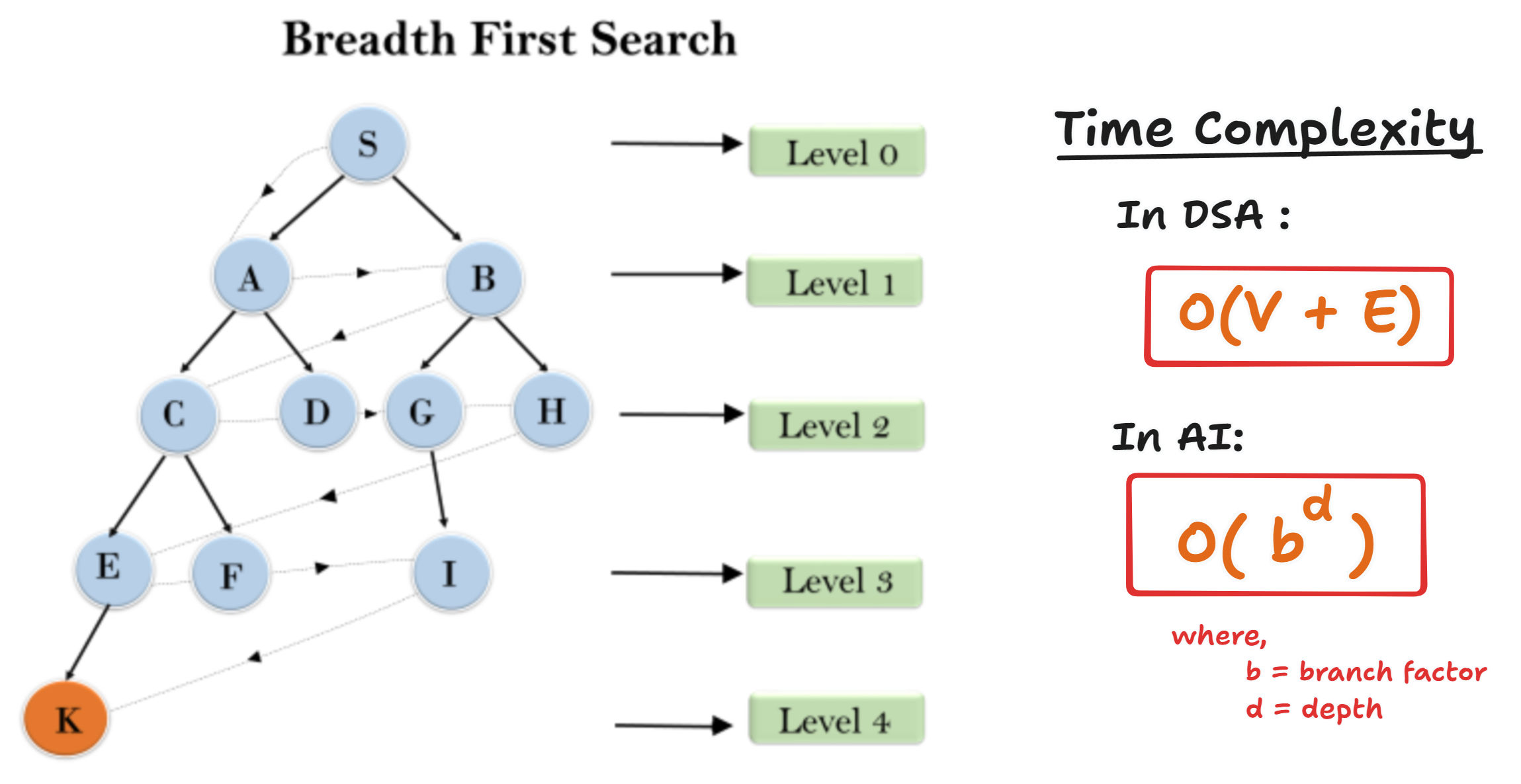
Breadth-First Search (BFS)

Explores all nodes at the current depth before moving deeper.
Uses a queue (FIFO).
Guarantees finding the shortest path in an unweighted graph.

Depth-First Search (DFS)

Explores one branch as deep as possible before backtracking.
Uses a stack (LIFO) or recursion.
May get stuck in infinite depth if cycles exist.

Uniform-Cost Search (UCS)

Expands the least-cost path first.
Uses a priority queue.
Guarantees optimal solution in weighted graphs.

Depth-Limited Search (DLS)

DFS with a depth limit.
Prevents infinite exploration in cyclic or deep spaces.

Iterative Deepening DFS (IDDFS)

Repeated DFS with increasing depth limits.
Combines the low memory usage of DFS with completeness of BFS.

BFS Algorithm (Steps)

Start from the source node and add it to a queue.
Dequeue a node, process it, and mark it visited.
Add all unvisited neighbors to the queue.
Repeat until goal is found or queue is empty.

Python Example – BFS

from collections import deque

def bfs(graph, start):
    visited = set()
    queue = deque([start])

    while queue:
        node = queue.popleft()
        if node not in visited:
            print(node, end=" ")
            visited.add(node)
            queue.extend(graph[node] - visited)

graph = {
    'S': {'A', 'B'},
    'A': {'C', 'D'},
    'B': {'G', 'H'},
    'C': {'E', 'F'},
    'D': set(),
    'E': {'K'},
    'F': {'K'},
    'G': {'I'},
    'H': set(),
    'I': {'K'},
    'K': set()
}

bfs(graph, 'S')

Output:

S B A G H C D I F E K

DFS Algorithm (Steps)

Start from the source node.
Explore one branch as deep as possible.
Backtrack if no further unvisited nodes are found.
Continue until all nodes are visited or goal is found.

Python Example – DFS (Recursive)

def dfs(graph, node, visited=None):
    if visited is None:
        visited = set()
    if node not in visited:
        print(node, end=" ")
        visited.add(node)
        for neighbor in graph[node]:
            dfs(graph, neighbor, visited)

graph = {
    'S': {'A', 'B'},
    'A': {'C', 'D'},
    'B': {'G', 'H'},
    'C': {'E', 'F'},
    'D': set(),
    'E': {'K'},
    'F': {'K'},
    'G': {'I'},
    'H': set(),
    'I': {'K'},
    'K': set()
}

dfs(graph, 'S')

Output:

S B H G I K A D C E F

Search Space & State Space Search

Search Space: The complete set of all possible states for a problem.
State: A configuration of the system at any point.
Initial State: Starting condition.
Goal State: Desired outcome.
Operators: Actions that transition from one state to another.
Transition Model: Defines how applying an action changes the state.
State Space Graph: Graph with nodes = states and edges = transitions.

Example: Map coloring problem

Variables = regions
Domains = (Red, Green, Blue)
Constraint = adjacent regions cannot share the same color

Heuristic Search

Heuristic search uses knowledge of the problem domain to guide search.

Heuristic Function (h(n)): Estimates cost from current state to goal.
Admissible Heuristic: Never overestimates → ensures optimal solution.
Inadmissible Heuristic: May overestimate → not guaranteed optimal.

A* Algorithm

Combines actual cost g(n) and estimated cost h(n):
```
  f(n) = g(n) + h(n)
```
Expands the node with the lowest f(n).
Guarantees optimal solution if heuristic is admissible.

Python Example – A*

import heapq

def a_star(graph, start, goal, heuristic):
    open_list = [(0, start)]
    g = {start: 0}
    parent = {start: None}

    while open_list:
        _, node = heapq.heappop(open_list)
        if node == goal:
            path = []
            while node:
                path.append(node)
                node = parent[node]
            return path[::-1]

        for neighbor, cost in graph[node]:
            tentative_g = g[node] + cost
            if neighbor not in g or tentative_g < g[neighbor]:
                g[neighbor] = tentative_g
                f = tentative_g + heuristic[neighbor]
                heapq.heappush(open_list, (f, neighbor))
                parent[neighbor] = node

graph = {
    'A': [('B', 1), ('C', 3)],
    'B': [('D', 1), ('E', 5)],
    'C': [('F', 2)],
    'D': [],
    'E': [('F', 1)],
    'F': []
}

heuristic = {'A': 6, 'B': 5, 'C': 2, 'D': 3, 'E': 1, 'F': 0}
print(a_star(graph, 'A', 'F', heuristic))

Output:

['A', 'C', 'F']

AO* (Anytime A*) Algorithm

The AO* (Anytime A*) algorithm is a search algorithm designed to find a solution quickly and then continue refining it as more time is available. Unlike the standard A*, which finds the optimal solution and stops, AO* can provide a “good enough” solution immediately and improve it iteratively. This makes it highly suitable for real-time applications, where a fast solution is critical but incremental improvement is beneficial.

AO* works by performing repeated searches with an increasing cost bound k, effectively exploring larger portions of the search space with each iteration.

Key Concepts

Anytime Performance: AO* can return a solution at any point during execution. The longer it runs, the better the solution it finds.
Iterative Deepening by Cost Bound: Instead of depth-limited iterative deepening, AO* uses a cost bound k. Each iteration searches for solutions whose total cost (f = g + h) is ≤ k.
Heuristic Function (h): Like A*, AO* relies on a heuristic h(n) to estimate the remaining cost from node n to the goal. A good heuristic improves efficiency.
Cost Function (f): The estimated total cost is f(n) = g(n) + h(n)
Bound Management: The cost bound k is increased after each iteration if no solution is found within the current bound.

**The AO* Algorithm Step by Step**

Initialize: Set the initial cost bound k and initialize the best solution as None.
Search within Bound: Perform an A*-like search but only expand nodes where f(n) ≤ k.
Check for a Solution:

If a solution is found within k, store it as the current best solution.
If no solution is found, increase k and repeat.

Iterate / Terminate: Repeat the search, increasing k each time. The algorithm can be terminated at any time. When it stops, the best solution found so far is returned. If allowed to run indefinitely, AO* will eventually find the optimal solution.

Adversarial Search (Games)

Applied in competitive domains (e.g., Chess, Tic-Tac-Toe).
Represented as a game tree where nodes = game states, edges = possible moves.

Minimax Algorithm

Two players:

Maximizer: tries to maximize score.
Minimizer: tries to minimize maximizer’s score.

Assumes both play optimally.

Alpha-Beta Pruning

Optimizes minimax by pruning branches that won’t affect final outcome.
Improves efficiency without changing result.

Python Example – Minimax (Tic-Tac-Toe)

def minimax(depth, is_maximizing):
    scores = {'X': 1, 'O': -1, 'Draw': 0}

    result = check_winner()
    if result is not None:
        return scores[result]

    if is_maximizing:
        best = -float('inf')
        for move in get_available_moves():
            make_move(move, 'X')
            best = max(best, minimax(depth + 1, False))
            undo_move(move)
        return best
    else:
        best = float('inf')
        for move in get_available_moves():
            make_move(move, 'O')
            best = min(best, minimax(depth + 1, True))
            undo_move(move)
        return best

Constraint Satisfaction Problems (CSP)

Defined as (X, D, C)

X = variables
D = domains (possible values)
C = constraints

Example: Sudoku

Variables = empty cells
Domain = (1,2,3)
Constraints = each row, column, block must have unique values

Solving CSP

Backtracking Search: Assign values step by step, backtrack when conflict occurs.
Constraint Propagation: Reduce possible values using rules (e.g., arc consistency).
Heuristics: Choose most constrained variable first (MRV), or variable affecting most others (MCV).

Planning, Control Strategies, and Implementation

Planning:

Classical Planning: Uses state-space search (e.g., STRIPS).
Probabilistic Planning: Handles uncertainty (e.g., Markov Decision Processes).
Hierarchical Planning: Breaks tasks into subtasks.

Control Strategies:

Reactive: Responds immediately to environment (e.g., obstacle avoidance in robots).
Deliberative: Plans ahead considering future states.
Hybrid: Combines both for efficiency.

Implementation:

Requires programming (Python, C++), frameworks (ROS), sensors, actuators.
Tested first in simulations before real deployment.

Game Playing AI

Types of Games: Board games (Chess), card games (Poker), video games, multi-agent strategy games.
Techniques:
Minimax with Alpha-Beta Pruning
Monte Carlo Tree Search (Go game)
Reinforcement Learning (AlphaGo, OpenAI Five).
Applications: Entertainment, finance (algorithmic trading), robotics (robot soccer), security (attack-defense strategies).

Summary Table – Search Techniques

Algorithm	Type	Data Structure	Advantage	Limitation
BFS	Uninformed	Queue	Finds shortest path	High memory use
DFS	Uninformed	Stack/Recursion	Low memory	May not find shortest path
UCS	Uninformed	Priority Queue	Finds least-cost path	Slow in large graphs
A*	Heuristic	Priority Queue	Optimal + efficient	Needs good heuristic
Minimax	Adversarial	Game tree	Optimal with perfect play	Exponential time complexity
Alpha-Beta	Adversarial	Game tree	Faster than minimax	Still expensive in large trees

Intelligent Agents and Search Techniques