Database Indexing & Hashing Techniques | Complete Guide to Query Optimization & Performance

Indexing & Hashing

In a database, information is stored as records. Each record contains a key field that uniquely identifies it (like a roll number identifying a student).

To find records efficiently — especially when dealing with large amounts of data — databases use a technique called indexing.
Indexing acts like the index section of a book, allowing us to quickly locate the required information without scanning every page.

Indices

An index is a data structure (like an index in a book) that allows faster retrieval of records from a database table.

It’s main purpose is to speed up read operations such as SELECT queries by minimizing disk access.

Each index entry contains:

Search Key: Copy of the attribute being indexed (e.g., Employee_ID).
Data Reference: Pointer to the location of the actual record in the disk block.

Types of Indexing:

Primary Index: Primary index is defined on an ordered data file. The data file is ordered on a key field. The key field is generally the primary key of the relation.
Secondary (Non Clustered) Index: Secondary index may be generated from a field which is a candidate key and has a unique value in every record, or a non-key with duplicate values.
Clustering Index: Clustering index is defined on an ordered data file. The data file is ordered on a non-key field.

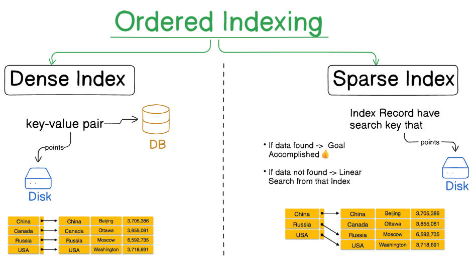
Ordered Indexing:

Dense Index: In dense index, there is an index record for every search key value in the database. This makes searching faster but requires more space to store index records itself. Index records contain search key value and a pointer to the actual record on the disk.
Sparse Index: In sparse index, index records are not created for every search key. An index record here contains a search key and an actual pointer to the data on the disk. To search a record, we first proceed by index record and reach at the actual location of the data. If the data we are looking for is not where we directly reach by following the index, then the system starts sequential search until the desired data is found.

Multi-Level Indexing:

When databases grow large, even the index itself can become too big to store in memory. To solve this, multilevel indexing is used.

Concept:

The index is divided into multiple smaller indexes.
The lowest level points to actual data.
The upper levels act as indexes of indexes.
The topmost level (root index) is small enough to fit in main memory.

Benefits:

Reduces disk access time.
Makes searching faster and scalable for large databases.

B-Trees

In database systems, dynamic indexing is essential for efficiently locating and managing records that are frequently inserted, deleted, or updated. The B-Tree (Balanced Tree) is one of the most efficient data structures designed for this purpose. It maintains balance dynamically while allowing quick data retrieval, insertion, and deletion operations.

What is a B-Tree?

A B-Tree is a self-balancing multi-way search tree where data is stored in nodes that can have multiple keys and pointers. Unlike binary search trees, each node in a B-Tree may contain multiple keys, which helps reduce the height of the tree and thereby minimizes disk I/O operations during searches.

Key Characteristics:

Records (or pointers to records) are stored in the nodes.
All leaf nodes exist at the same level, ensuring balance.
Nodes split or merge automatically during insertions and deletions to maintain uniform height.

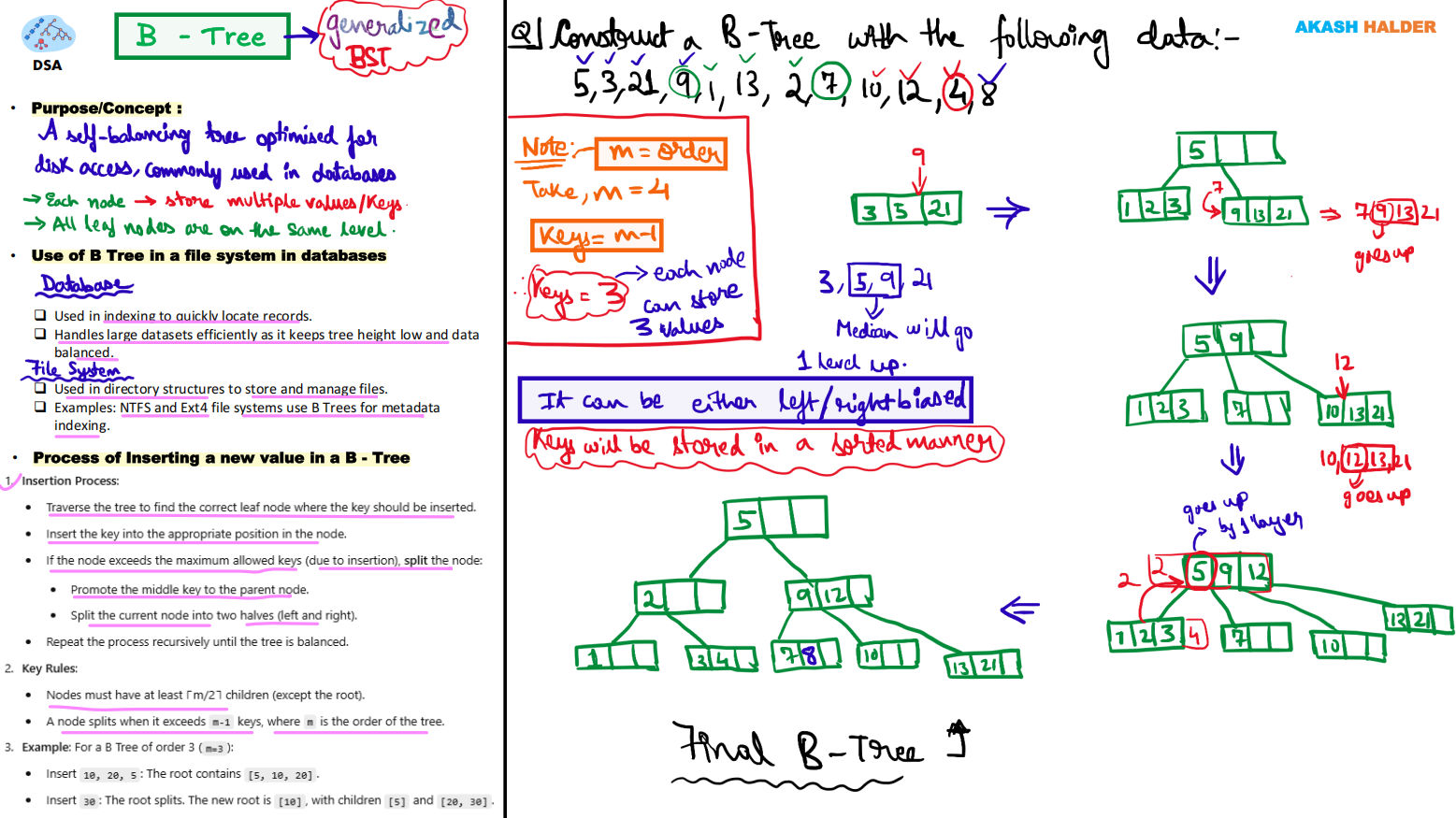
Working of a B-Tree

1. Nodes and Keys

Each node can have multiple keys and pointers. The number of keys and pointers is determined by the order (p) of the B-Tree.

A node can have up to p pointers and p−1 keys.
Keys are arranged in ascending order.

2. Balanced Structure

The B-Tree is always balanced, meaning the path length from root to any leaf node is the same.

3. Search Operation

The search starts from the root node.
Based on key comparisons, appropriate pointers are followed down to lower levels.
The process continues until the desired record is found or confirmed absent.

Key Properties of B-Trees

Property	Description
Order (p)	Maximum number of child pointers per node
Keys per Node	Up to p−1 keys arranged in ascending order
Balance	All leaf nodes appear at the same level
Minimum Occupancy	Each node is at least half full (except the root)
Linked Leaves	Leaf nodes may be linked for sequential access

Example Structure of a B-Tree

For a database with:

Order (p): 23
Fan-out: 16

The growth pattern is as follows:

Level	Nodes	Keys	Pointers
Root (Level 0)	1	15	16
Level 1	16	240	256
Level 2	256	3840	4096
Leaf Level	4096	61,440	—

This structure efficiently supports over 65,535 records using just three levels, resulting in very fast search operations.

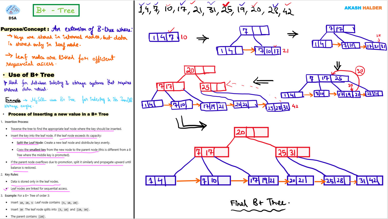
B+ Trees: The Improved Version

A B+ Tree is an enhanced form of a B-Tree, optimized specifically for indexing. The primary difference is that data records are stored only in the leaf nodes, while internal nodes store only keys and pointers.

Structure:

Internal Nodes: Contain only keys and pointers to child nodes.
Leaf Nodes: Contain actual data records or pointers to them.
Linked Leaves: Leaf nodes are linked to allow range queries and sequential access.

Key Properties of B+ Trees

Property	Description
Internal Nodes	Contain only keys and child pointers
Leaf Nodes	Contain actual records or record pointers
Order (p)	Each internal node can have up to p pointers and p−1 keys
Linked Leaves	Enables fast range queries
Balanced	Automatically maintains balance during insertions/deletions

Example Structure of a B+ Tree

Assume:

Key size: 9 bytes
Pointer size: 7 bytes (record), 6 bytes (block)
Block size: 512 bytes

Derived capacity:

Internal Node: 34 keys, 35 pointers
Leaf Node: 31 records

Level	Nodes	Keys	Pointers
Root	1	22	23
Level 1	23	506	529
Level 2	529	11,638	12,167
Leaf Level	12,167	255,507	—

Thus, the structure can manage over 255,000 records with only three levels, offering extremely efficient access.

Advantages of Dynamic Multilevel Indexing

Advantage	Explanation
Automatic Balancing	Nodes split or merge automatically, maintaining a balanced structure.
Efficient Searches	Reduced tree height leads to faster searches.
Quick Updates	Insertion and deletion are handled efficiently.
Scalability	Supports large datasets without performance degradation.

Real-world Applications

Domain	Use Case
DBMS	Indexing tables for fast query performance
File Systems	Efficient file access and directory management
Search Engines	Optimized keyword and document indexing
Operating Systems	Directory and metadata indexing

Difference Between B-Trees and B+ Trees

Feature	B-Tree	B+ Tree
Data Storage	In all nodes	Only in leaf nodes
Data Retrieval	Slower for range queries	Faster due to linked leaves
Tree Depth	Deeper	Shallower
Range Queries	Less efficient	Highly efficient
Use Cases	General-purpose indexing	Database and file system indexing

Conclusion

B-Trees and B+ Trees play a critical role in dynamic multilevel indexing by maintaining balanced, efficient search structures.

B-Trees store data in all nodes and provide fast direct access.
B+ Trees, optimized for indexing, store records only at leaf nodes, ensuring faster sequential and range-based searches.

Hashing

In large database systems, searching through multilevel indexes can be time-consuming and storage-intensive. Hashing offers an efficient alternative by providing direct access to data records using a hash function. Instead of traversing index structures, hashing computes the storage address of a record directly based on its key value, leading to constant-time data retrieval.

Concept of Hashing

Hashing uses a hash function (h) that takes a search key (K) as input and returns an address or bucket number where the record is stored. This allows the database to quickly locate records without performing multi-level index lookups.

Components of Hashing

Hash Function (h): Maps a search key to a specific bucket address.
Bucket: The unit of storage that typically corresponds to a disk block. Each bucket can store one or more records.

Formula:

Bucket address = h(K)

Hash Organization

Component	Description
Bucket	Logical storage unit that holds one or more data records. Usually corresponds to a physical disk block.
Hash Function	A deterministic mapping function `h(K)` that converts search keys into bucket addresses.

Example: If h(K) = K % 4, possible bucket addresses are 0, 1, 2, 3. Records are placed into one of these four buckets.

Static Hashing

In static hashing, the number of buckets remains fixed. The same hash function always produces the same address for a given key. While efficient for stable data sizes, static hashing struggles when the database grows or shrinks.

Operations in Static Hashing

Insertion Compute the bucket address using the hash function and store the record in that bucket.
```
address = h(K)
```
Search Use the same hash function to locate the bucket and retrieve the desired record.
Deletion Locate the record using the hash function and remove it from the corresponding bucket.

Bucket Overflow and Collision Handling

Bucket overflow occurs when multiple records hash to the same bucket and it becomes full. This situation is known as a collision. Two primary strategies handle collisions:

1. Overflow Chaining (Closed Hashing)

When a bucket is full, an overflow bucket is created.
The new bucket is linked to the original one.
The chain continues as needed.

This mechanism is suitable when data access patterns are unpredictable but not excessively dense.

2. Linear Probing (Open Hashing)

When a collision occurs, the system searches for the next available bucket sequentially.
The record is placed in the nearest free slot.

This method keeps all data within the main hash table, avoiding external overflow buckets.

Dynamic Hashing

Dynamic hashing (also called extendible hashing) resolves the limitations of static hashing. It allows the hash structure to expand and shrink dynamically as data grows or decreases.

Unlike static hashing, dynamic hashing uses a hash function that can produce a large number of potential values, but initially utilizes only a subset.

Organization of Dynamic Hashing

Dynamic hashing uses a directory and a hash function that produces binary hash values.

The prefix bits of the hash value determine the bucket address.
Each directory entry maintains a depth value, representing the number of bits used.
When a bucket overflows, the system increases the depth and doubles the directory size, allocating new buckets accordingly.

Example

If a hash value uses 3 bits, it can address 2³ = 8 buckets. If all 8 buckets are filled, the system increases the depth to 4 bits, allowing 16 buckets.

Operations in Dynamic Hashing

Operation	Description
Querying	Use prefix bits (as defined by the depth) to compute the bucket address and fetch the record.
Insertion	Compute bucket address using `h(K)`. If the bucket is full: add new buckets, increase depth, and recompute hash values.
Deletion	Locate and remove the record. If a bucket becomes empty, the system may merge it with another to reduce space.
Update	Locate record using the hash function and update in place.

Comparison: Static vs Dynamic Hashing

Feature	Static Hashing	Dynamic Hashing
Bucket Count	Fixed	Grows/Shrinks dynamically
Performance	Degrades as database grows	Maintains efficiency as size changes
Collision Handling	Requires chaining or probing	Handled through directory expansion
Flexibility	Less flexible	Highly adaptive
Use Case	Suitable for small or stable databases	Ideal for large, dynamic databases

Limitations of Hashing

Not efficient for range queries (e.g., finding all records between two values) because hash functions do not preserve key ordering.
Works best when data keys are random and uniformly distributed.
Hash function design is crucial; poor hashing may lead to clustering and performance degradation.
Has a higher implementation complexity compared to traditional indexing.

Advantages of Hashing

Advantage	Description
Fast Access	Constant-time data retrieval (O(1)) for direct lookups.
Dynamic Adaptability	Dynamic hashing grows with the database.
Reduced Disk I/O	Minimizes index traversal.
Efficient Storage	Buckets are reused efficiently, minimizing space waste.

Conclusion

Hashing is a powerful data organization technique that enables direct record access without traversing hierarchical indexes.

Static hashing provides constant-time lookup but lacks scalability.
Dynamic hashing overcomes this by expanding and contracting in response to data volume.

Although hashing is not suitable for ordered or range-based queries, it is exceptionally efficient for random access patterns, making it widely used in database indexing, symbol tables, and hash-based file systems.